Regression Intelligence practical guide for advanced users (Part 2)
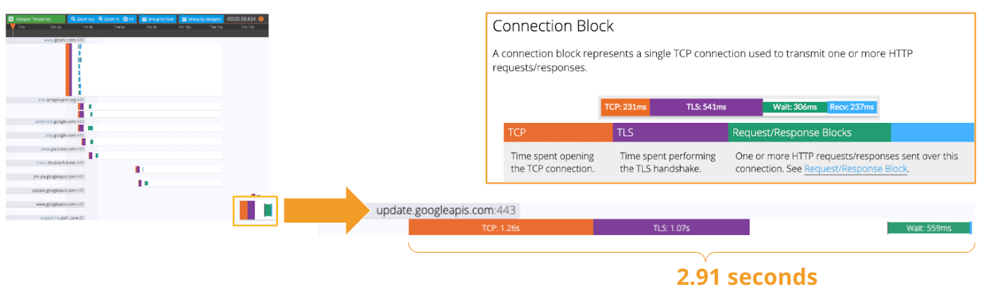
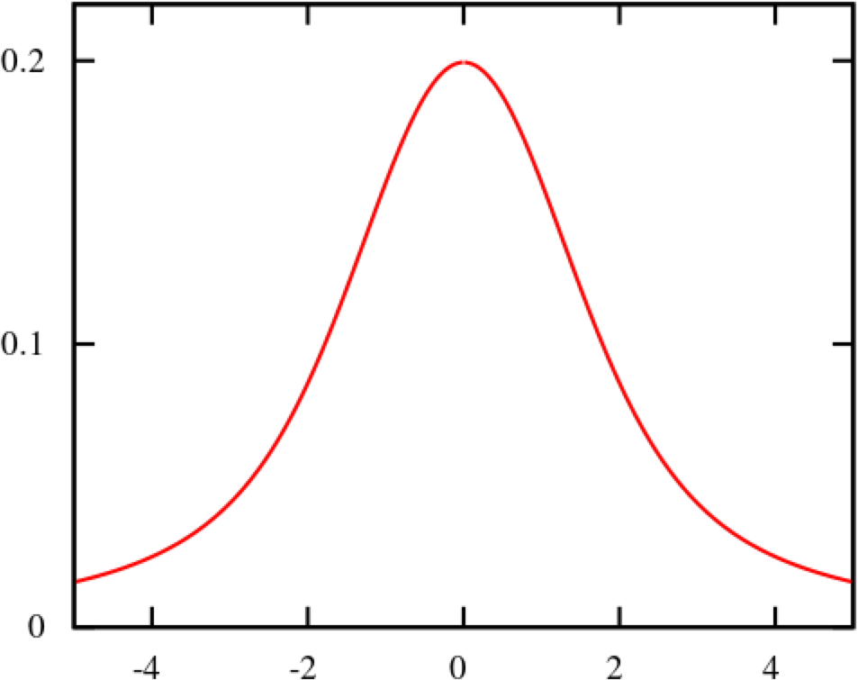
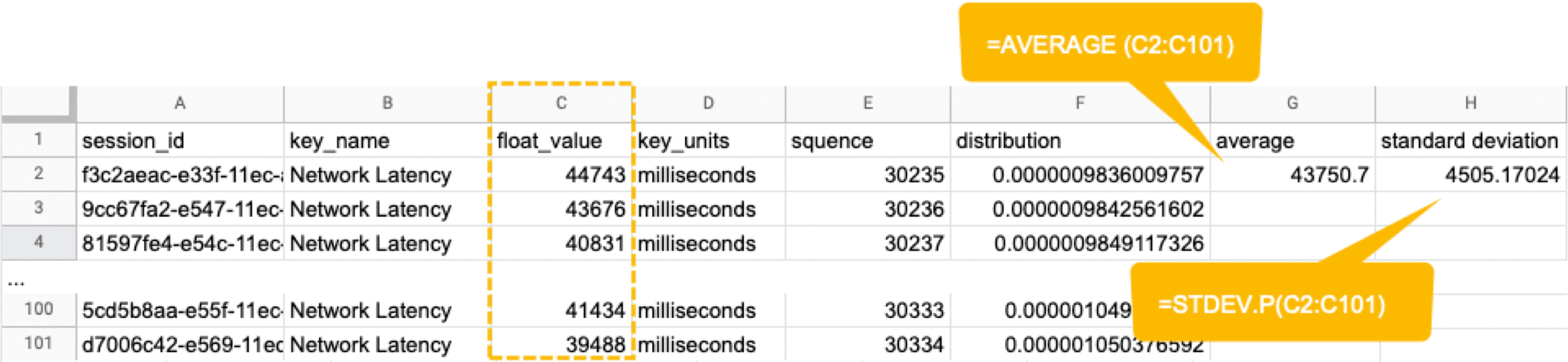
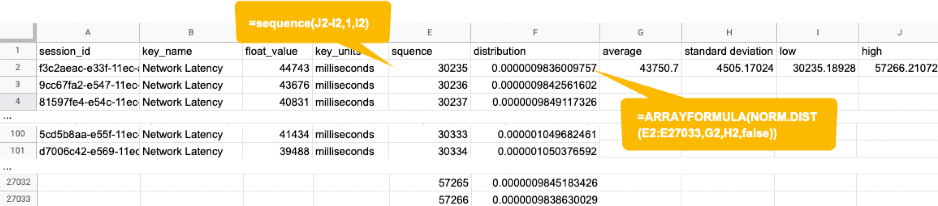
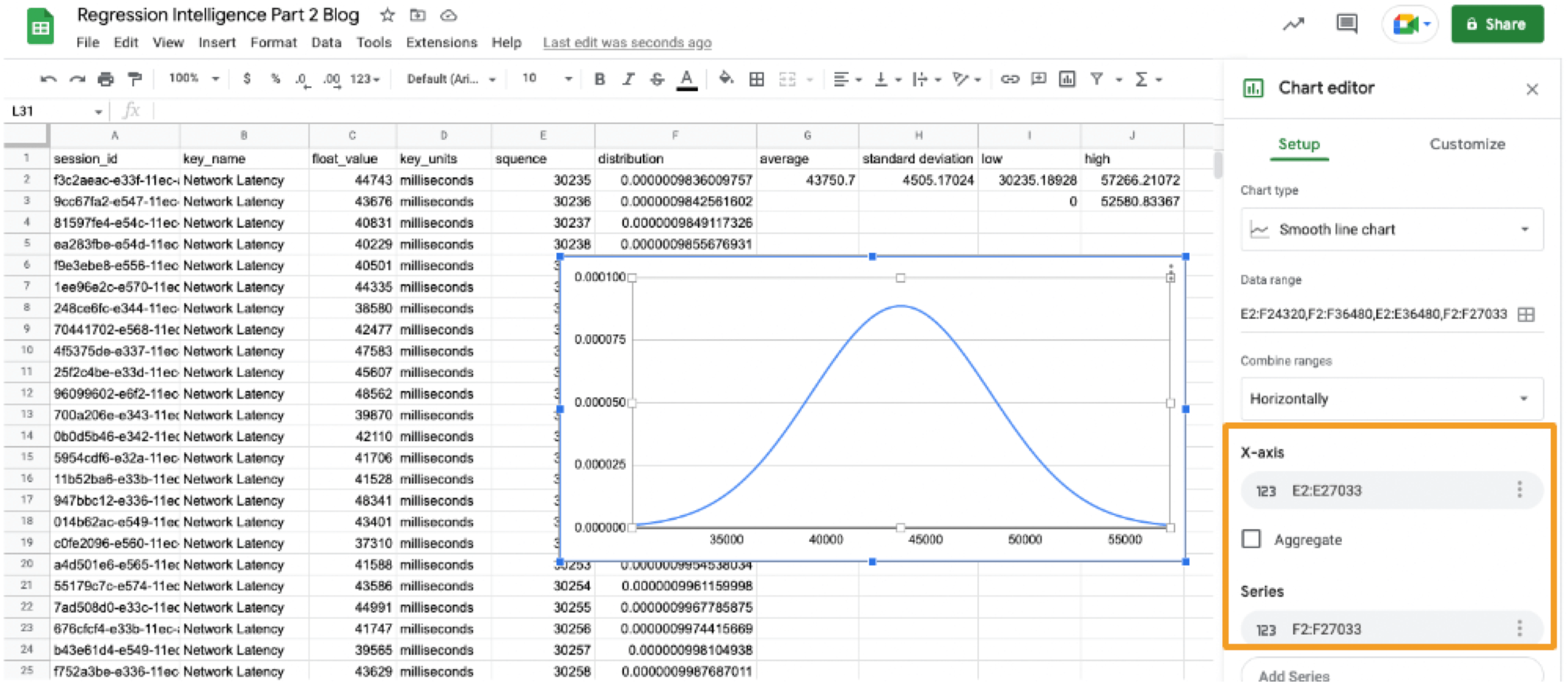
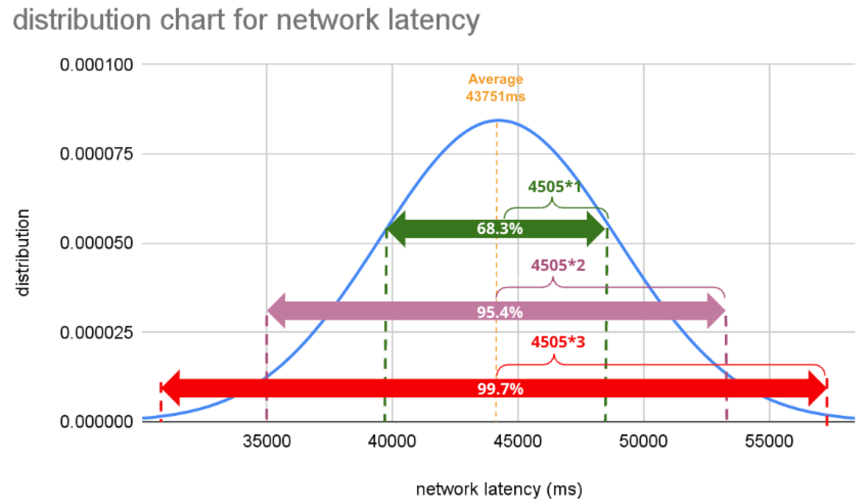
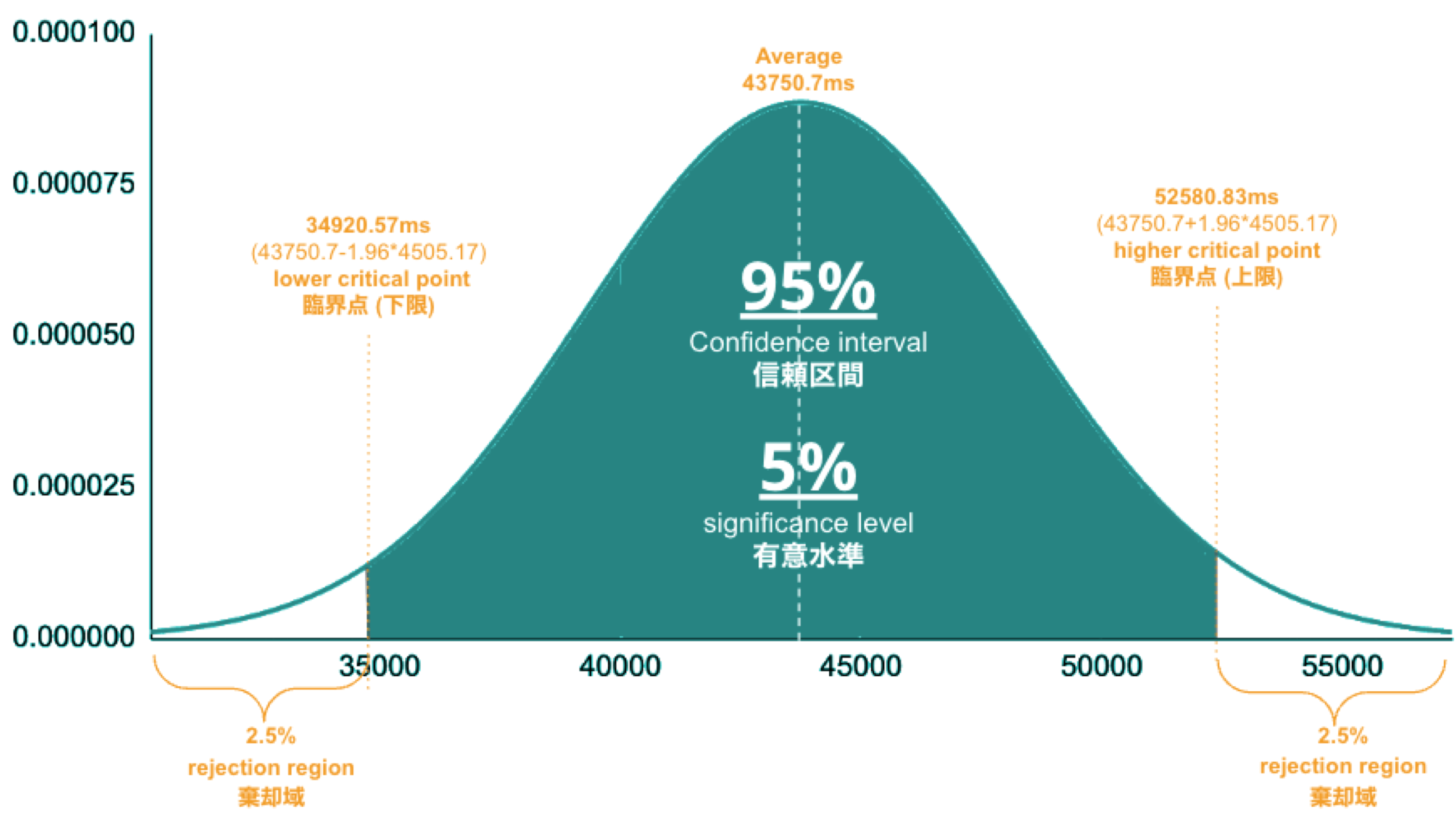
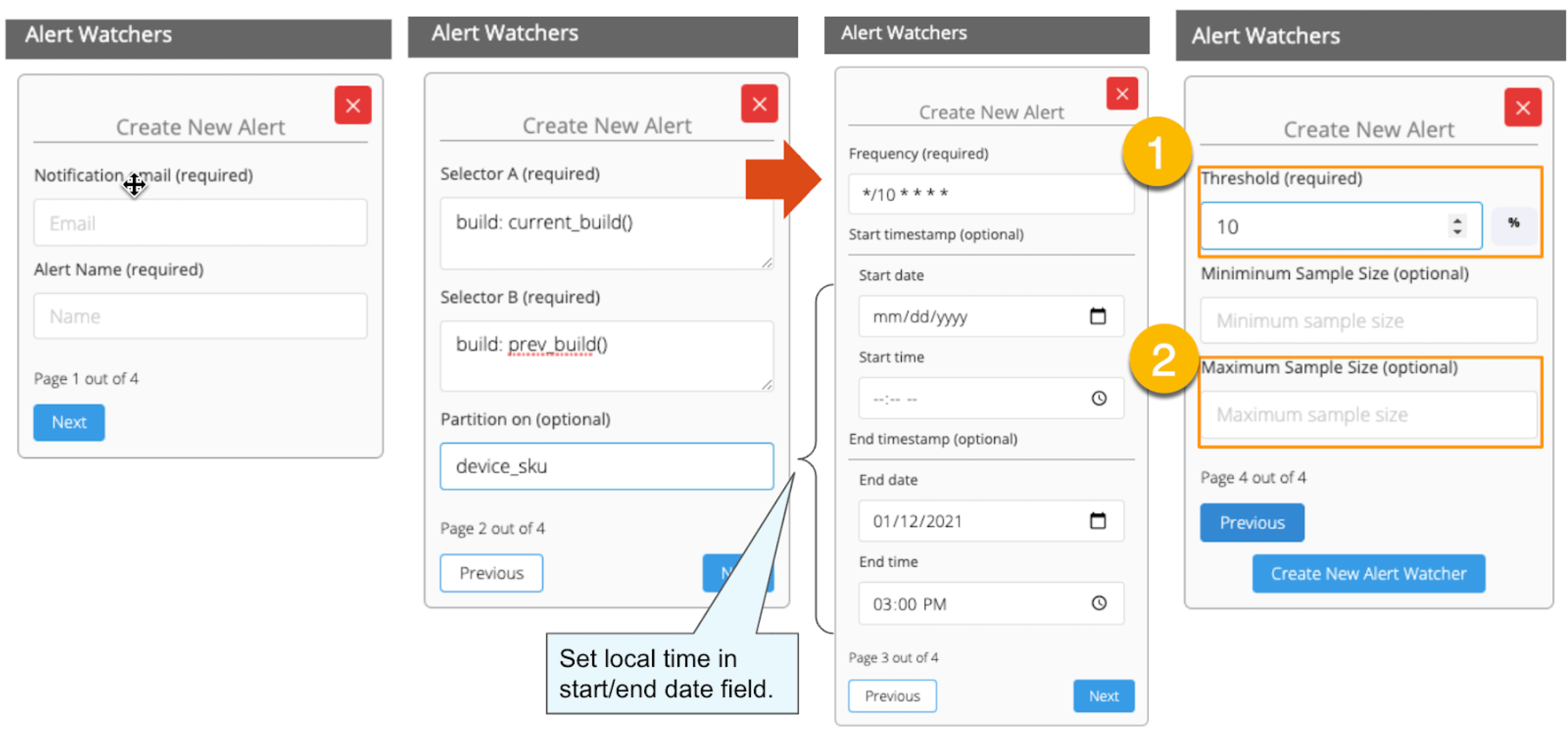
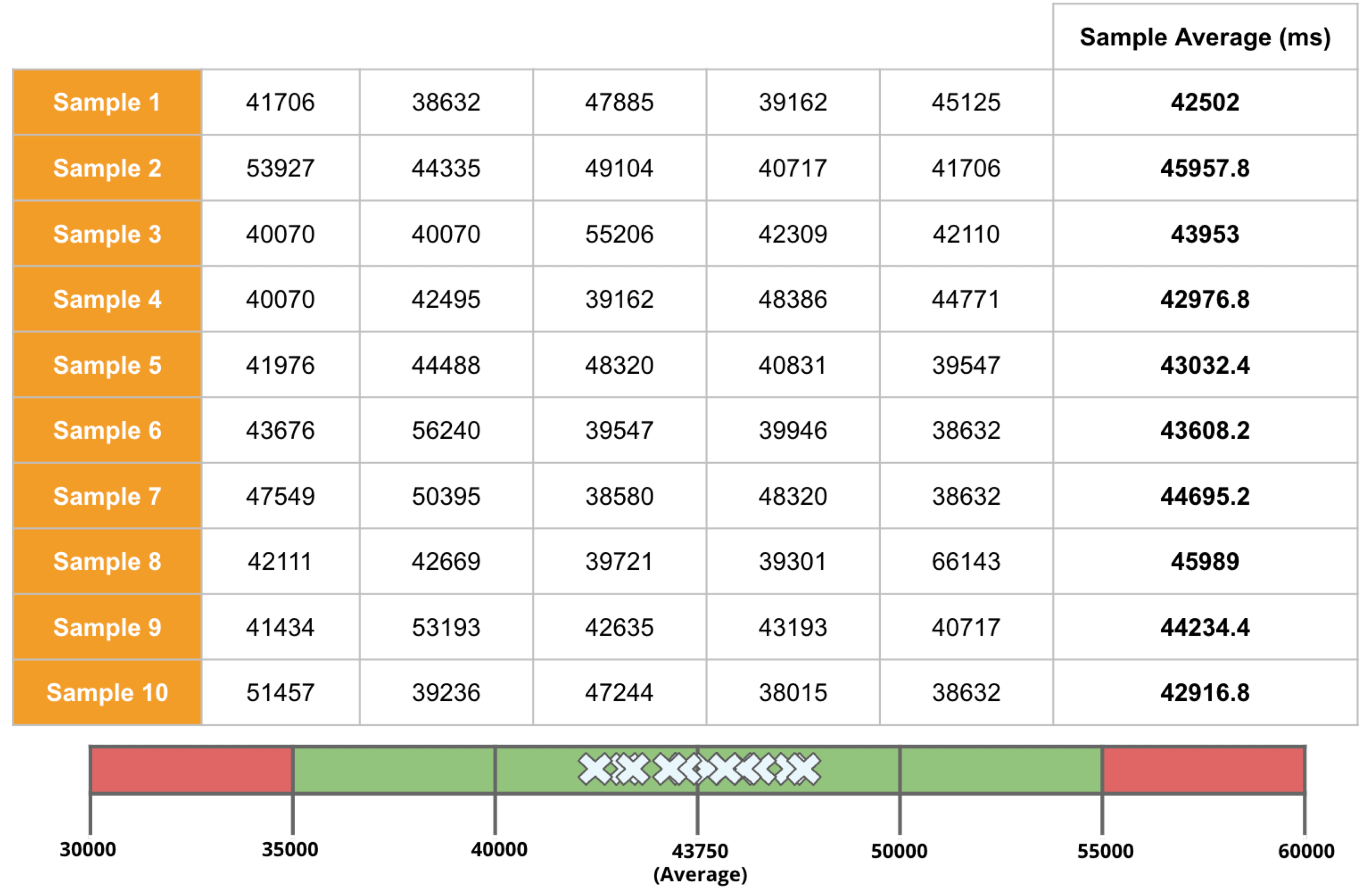
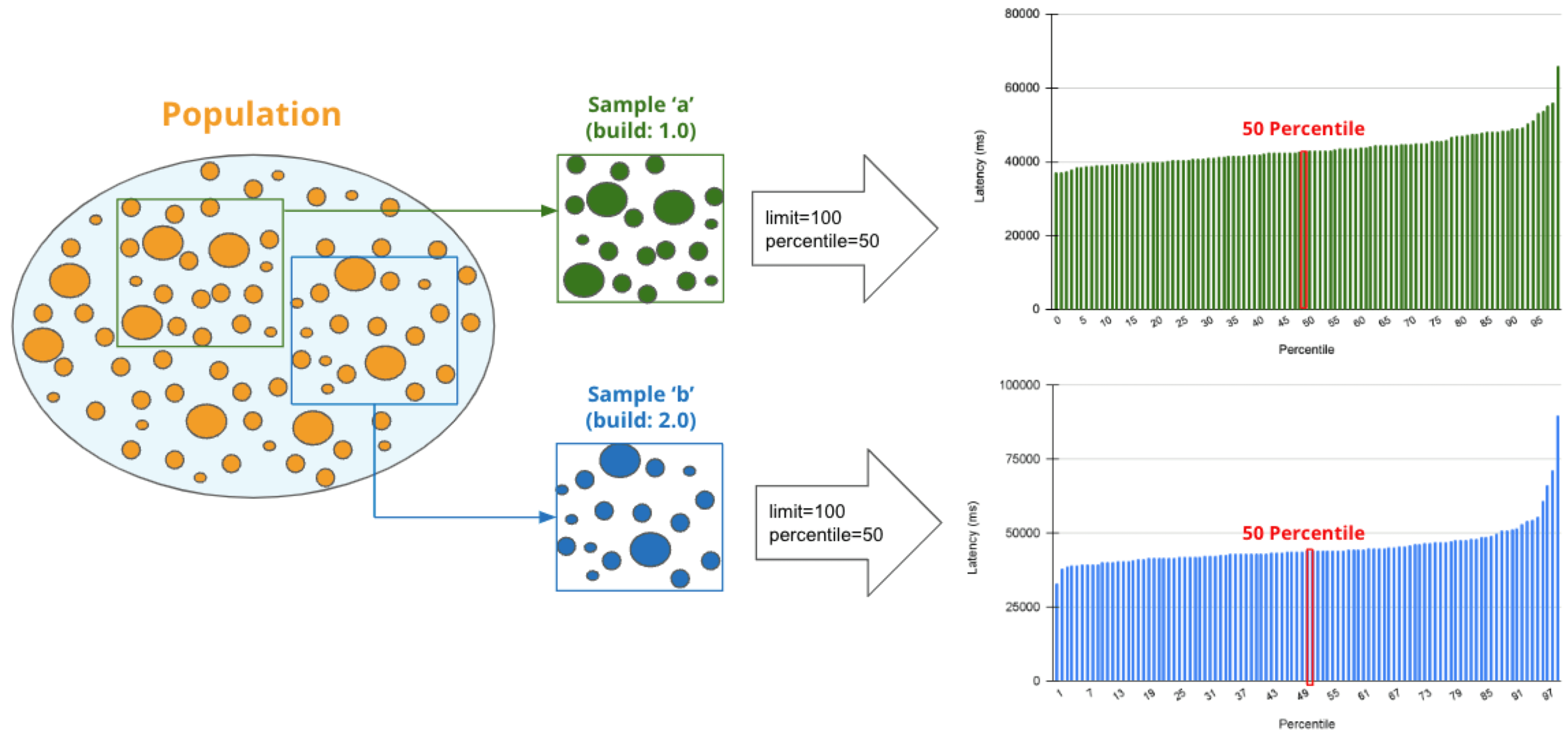
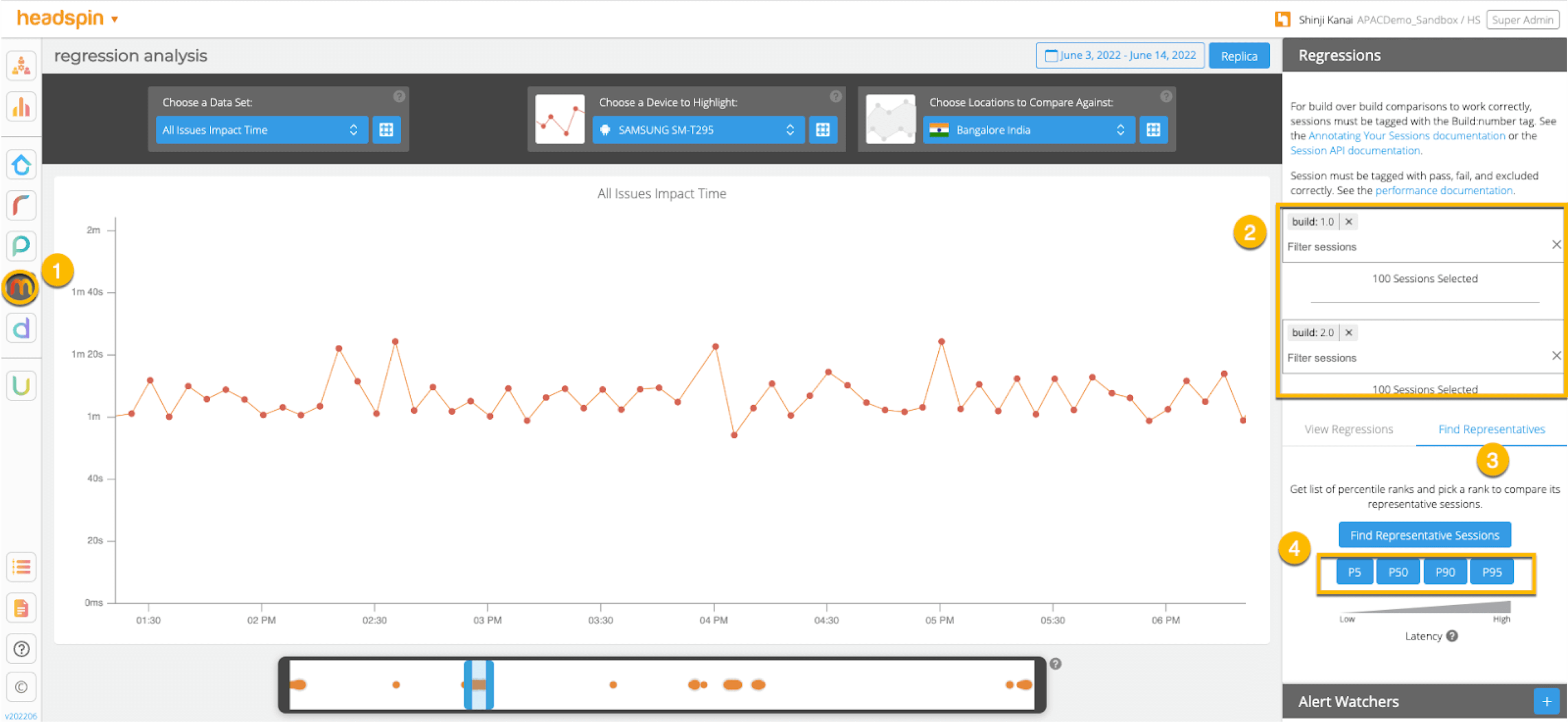
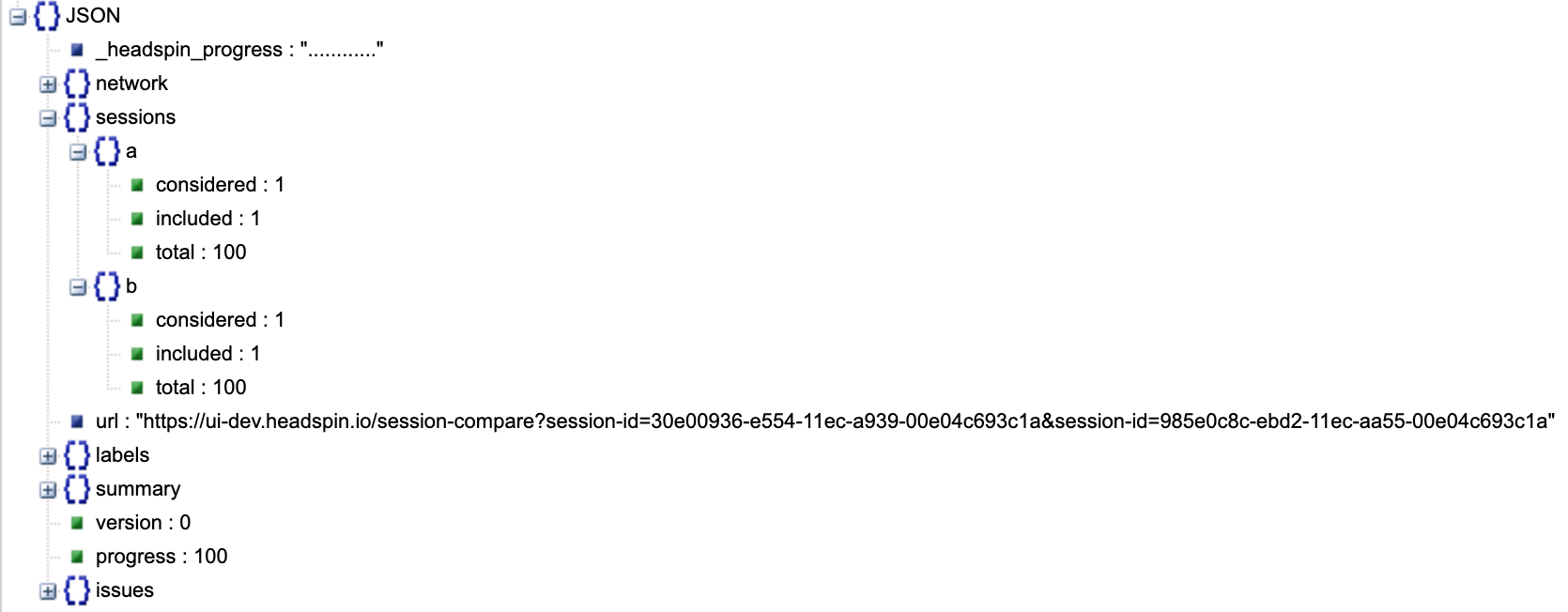
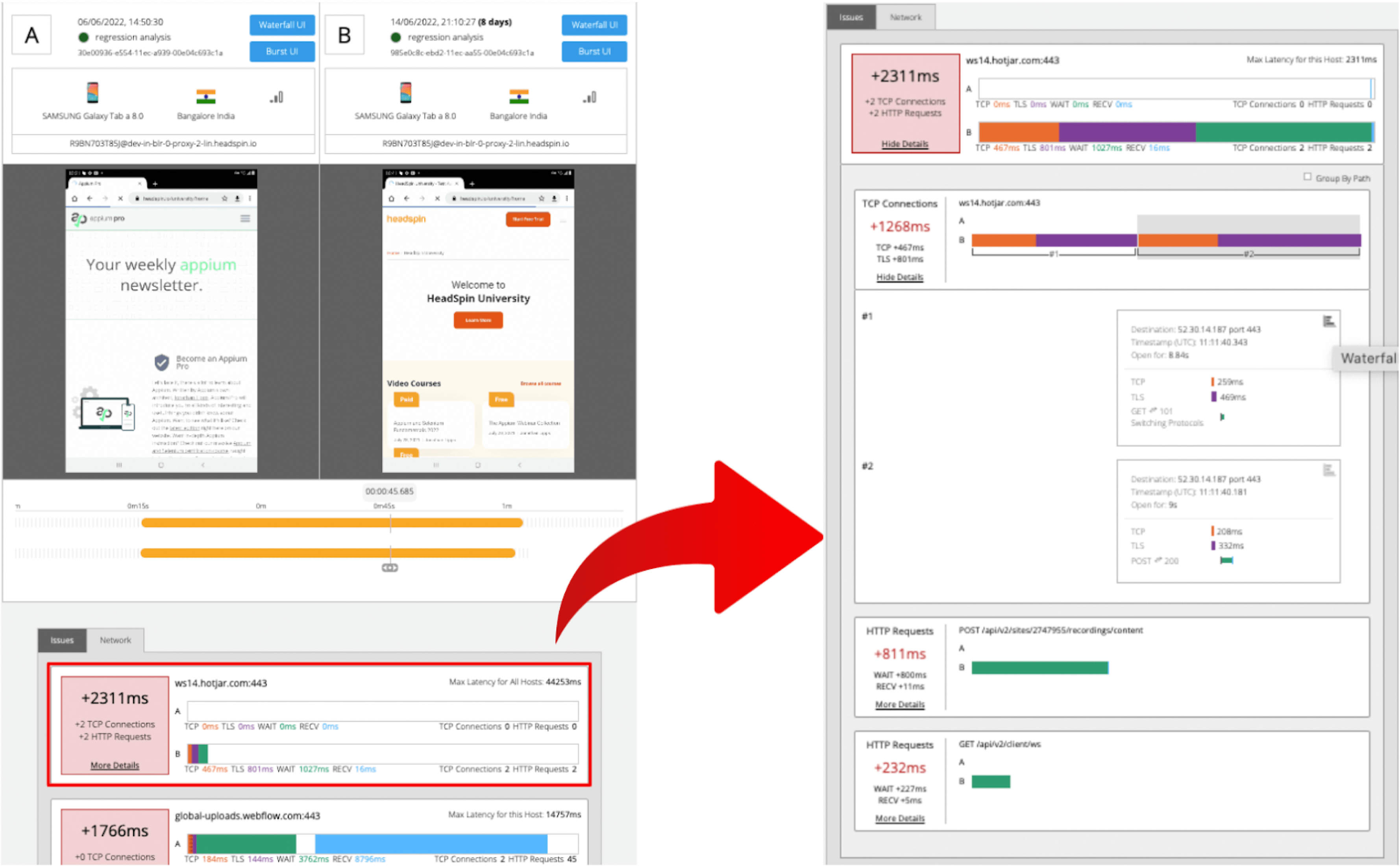
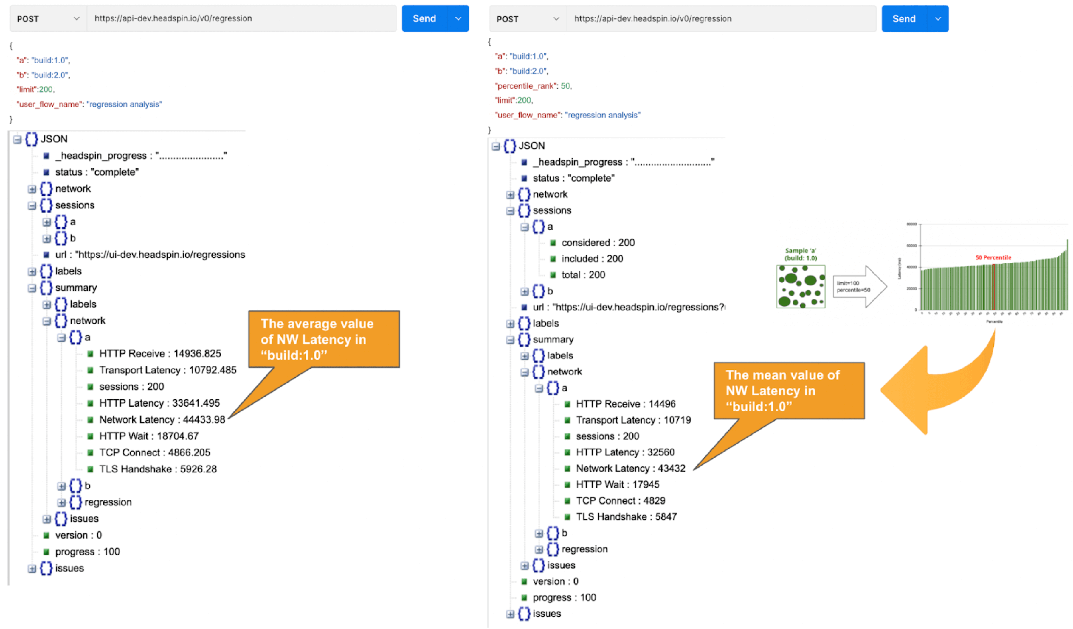
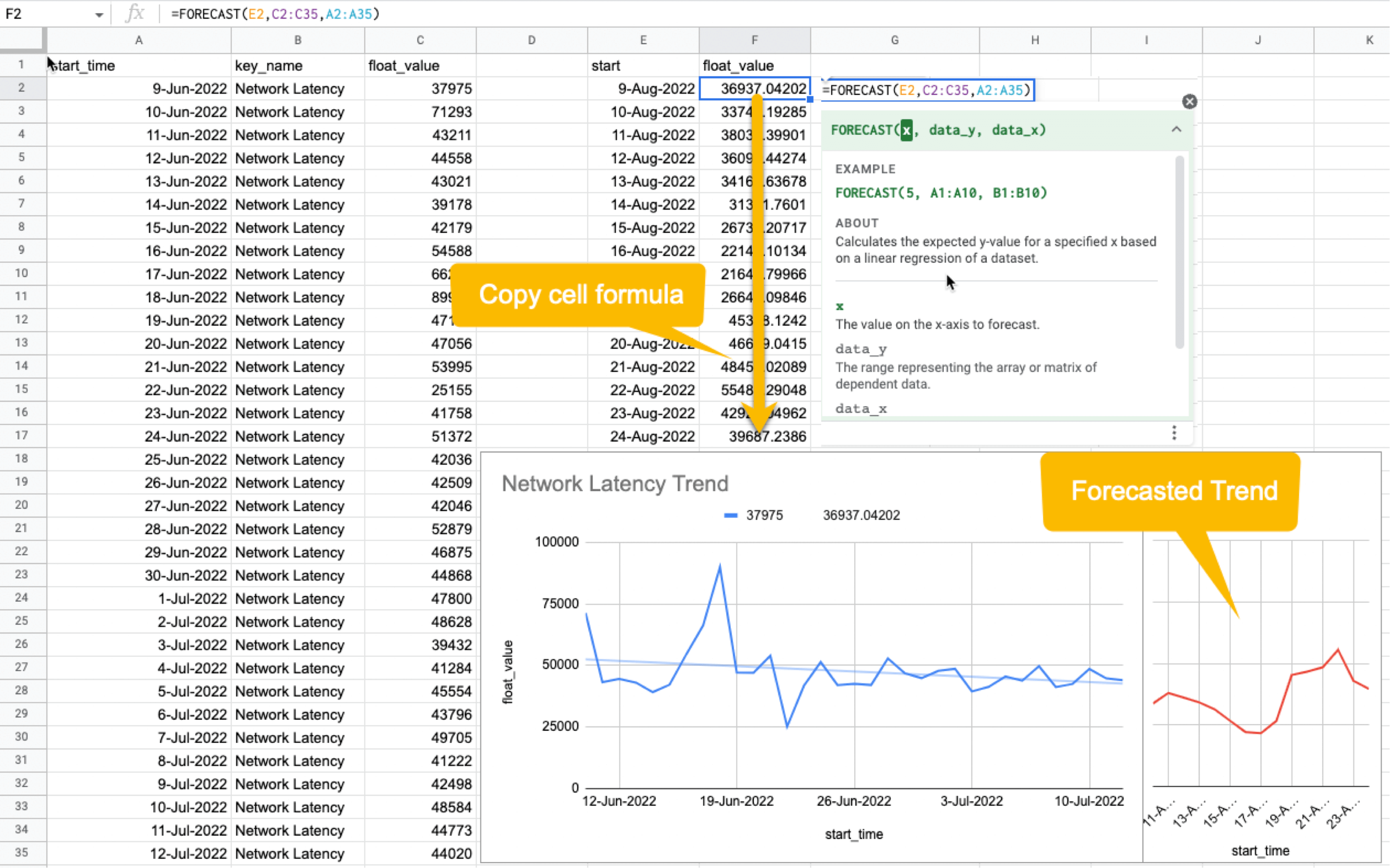
Welcome to the concluding of a two-part serial, & quot; Regression Intelligence practical usher for advanced users & quot;!, we walked through the virtual use of Regression Intelligence and Grafana through setting up custom KPIs and alerts. In this terminal serial, you will memorise about statistical supposition screen to solve network latency using. Many subscriber of this blog would have a solid knowledge of networks. However, I suppose not many see the importance of statistical theory try in get fixation. To see, here is a question for you! How would you respond the following question? Q) Given v1.0 and v2.0 of a mobile application, you liken the two builds to see execution differences on a specific operation. The outcome showed that v1.0 took 44s and v2.0 occupy 54s; v2.0 took 10s longer on average. Can we say a regression hap? Perhaps some people will say, & quot; No problem, if it is solely 10 seconds & quot;, while others will say, & quot; No, no, it & # x27; s a regression because it increased by an average of 10 seconds & quot;. And some might say, & quot; Try another test to see if the gap disappears & quot;. Opinions are divided… In the first half of this blog, I will introduce the statistical concepts that lead to a legitimate answer to this question. In the second half, you will configure Regression Intelligence and apply the construct learnt in the first one-half. Toward the end, you will be exposed to knock-down comparing and prediction methods that you can employ in your network investigation and beyond. Below are the topics covered in this blog. Excited? Let ’ s take a look at the initiatory issue! Network Latency generally intend the time it takes for a data packet to travel back and forth between the client and host. When capturing network traffic with HeadSpin, round-trip times can be accumulate in particular for each HTTP/HTTPS transaction. See the diagram below, which shows the time lead to complete a transaction and its breakdown by waiting case. In this case, 2.91s counts towards Network Latency (KPI). When applications and service send and find large parcel, even slight hold on a transaction-by-transaction basis can leave in sensed slow performance and stress users. The encroachment of network latency on business differs across industries and business sizes, but here are some examples: None of the above can be ignore. As you know, today & # x27; s networks are complex and globose, dwell of variously tie technologies such as VPNs, ISPs, CDNs, 4G/5G, Cloud and Edge and more. How can delays and anomalies in this vast network, which can occur anywhere at any time, be find? The reply is continuous data collection. The purpose of data assemblage in latency detection is to figure out the valid values of your network when healthy. Once you know what valid values for your mesh are, you can determine whether the network is in good or bad stipulation by appear at numbers. But the question is, what delineate the “ valid ” values you guess are valid? That ’ s where statistics comes into play! In the next topic, I will explain how to make and read the normal dispersion needed to identify these valid value. By the way, this is off-topic, but it ’ s best to use automation in data collection, as it requires a large amount of data to name the optimal state of your network. Also, to accumulate realistic results, automation should run on the exploiter & # x27; s edge device (e.g. Mobile, browsers). Here for a recommended course to learn the bedrock of Appium and Selenium. The normal dispersion is the near important probability distribution for understanding statistic. The gens comes from the fact that it is a probability distribution that applies easily to various phenomena such as & quot; normal & quot; (= & quot; cliche & quot; or & quot; normal & quot;) nature and human demeanor and characteristics. The graph is a symmetric (bell-shaped) curve, as shown in the diagram below. All events handled by HeadSpin fit this normal dispersion. Even if there are some exceptions, when the universe grow to a certain extent, it is know to approach a normal distribution according to theFundamental Limit Theorem. Follow the link to cognise the possibility better. For now, no more difficult words! We will make a normal distribution based on Network Latency (KPI) and see it!!! The following instructions assume you have a & quot; regression analysis & quot; user flow that already exists which storage 100 sessions tagged with “ build:1.0 ”. The first pace is to extract the Network Latency (KPI) from the Postgres database. Use the following SQL for recovery. For information on how to access the Postgres DB, check. Below is the result of running SQL above, which can also be accessedhere as sample datum. Next, we will figure the average and standard divergence of the Network Latency in column C. Only these two parameters are required as input to make a normal distribution afterwards. Here, we will use Google Sheet to run some math. See the image below showing how to forecast the average and standard deviation in column G and H, respectively. By the way, have you ever wondered what the standard deviation is? It is a magic number. It state us how far away from the average value, the information point are dust. The calculation is simple and can be done manually; you subtract the average value of 43750.7 from each value in column C, sum up all, and fraction the sum by the total number (in this instance, 100). Got the idea? The larger the standard departure is, the farther aside from the average value the information you have in hand are. That ’ s all we need to know. Next, in the column G and F, we enrol the figure representing the bell shape & # x27; s leftmost (minimum) and rightmost (maximum). They will be used later when create the chart. You will curtly cognise why we use the population norm ±3 * (Standard Deviation) in the formula. Next, add the E and F column: In the E column, you allot a serial bit that increases by one from low to high. Then, in the F column, enroll the result of theNorm.Dist part, which we will convert to a normal distribution next. The Norm.DIST purpose takes two argument as stimulus, the average value and standard deviation. The final numbers in column F imply the chance of each KPI value in column E. Finally, select all value in E and F columns to create a & quot; Smooth line chart & quot;. This produces a normal dispersion, as evidence below. So what does this normal dispersion recite us? Looking at this chart, you can tell the probability that specific meshing latency will occur. For representative, the likelihood of a net latency of 60 mo to happen is less than 0.3 %. Where does 0.3 % come from? See below. There is a known truth (called68-95-99.7 rule) about the normal distribution. That is if we cognize how far away from the population average the item-by-item data is, in standard deviation units, you can determine the rarity of the datum. Don & # x27; t think too much but recollect the three commonly used separation and their chance (=interval percentages), which are presented below: SUSA automates exploratory testing with persona-driven behavior, catching bugs that scripted automation misses. , we set the & quot; unacceptable battery usage & quot; KPI threshold to 10 % with no logical reason. Often, relying on feeling or suspicion in determining a doorway is not a good idea. Thus we use statistics. So the question is, how can we find the statistically correct threshold? To know the answer, you need to understand four concepts; significance level, confidence interval, critical point, and rejection region. Sounds hard? Not at all. See the diagram below. So, the correct way to find an optimum threshold is three stairs; 1. create a normal distribution from the large data you collected from your network, 2. decide your signification level, and 3. figure out a critical point in your dispersion. In this example, 52580.83ms (≈52.6 s) is the threshold we like for set alerts later. Now, let us return to the question posed at the beginning. Q)Given v1.0 and v2.0 of a mobile application, you compared the two builds to see performance differences on a specific operation. The result showed that v1.0 took 44s and v2.0 took 54s; v2.0 took 10s long on average. Can we say a fixation occurred? A)The resolution isYESif the significance level is 5 %. It is because If the significance level is set to 5 %, the upper critical point is 52.6s, and 54s falls in the upper rejection area; hence the 10s gap is considereda significant difference. But if the import level is 1 %, the answer isNObecause the upper critical point shifts to 57.3 % and 54s can stay inside the confidence interval; hence the 10s gap is not considered important. Remember that the outcome will thus vary count on the significance level you set. The hypothesis testing method used here is called Z-test in the statistics existence; Z-test is a eccentric of statistical hypothesis testing that uses a normal distribution. This concept has be applied in diverse battlefield, including economics and medicine. It is an effective concept, so if you don & # x27; t know about it, this is an fantabulous chance to master it. We experience explicate this without using complicated terminology, but if you would like to know more about Z-test, please hunt & quot; Z-test & quot;, & quot; null and alternative hypotheses & quot;, and & quot; statistical hypothesis test & quot;. Moving on, we will set alarum using the optimum threshold identified and learn some more statistics concepts. In this section, we will set up regression alerts and implement continuous monitoring via Web UI; please refer to for setting a watcher via the API and applying it to custom KPIs other than ‘summary.network.regression. ” Network Latency ”’. As of this writing, the Web UI only indorse the & quot; Network Latency & quot; KPI for fixation tracking. Navigate to a user flow and follow the diagram below to set alerting. For chooser and cron expression, refer to the relevant tables in. 1. The threshold value is 5 %, calculate using the following formula: 2. Maximum Sample Size is the sample/limit size, the number of sessions to analyse. The nonpayment value for limit sizing is 15. You may inquire, “ Why 15? Can it be set high? ”. This answer is closely related to statistics, so let me reply it below in detail. A) As you guess, the high the number of sessions include in the analysis, the better the accuracy is. You can achieve the best truth by hold the entire population included in the analysis; this is called a & quot; full survey & quot; as opposed to a & quot;sampling study& quot;. Doing a & quot; full resume & quot; prevents the intrusion of a & quot;sample error& quot;, which is the dispute between the sample norm and the universe average. However, in many cases, the universe tends to be very large. The analysis time can exceed tens of minutes or an hour if the sampling size exceeds respective hundred or yet thousands. This oft makes it not ideal to carry out a & quot; full survey & quot;. Not only that.The population sizes fluctuate over time. The sessions be 100 today will be 200 tomorrow. You can increase the limit size programmatically, but not a full idea from a maintenance and operation perspective. A & quot; sample survey & quot; approaching is therefore preferred. The concept of random sample is essential to minimise & quot; sample error & quot;. One well-known statistical truth is that & quot;the norm of willy-nilly selected samples approaches the population norm& quot;. The diagram below illustrates this construct in an intuitive and easy-to-understand manner. In the example above, the sample size is 5. There are 10 sample averages, and you see them all gather near the population norm of 43,750ms. Regression Intelligence pseudo-randomly picks 15 sampling by default. The “ pseudo-randomly ” means as long as the tag/selector and the sizing of the population remain unaltered, the same sample will be select each time; if new sessions are added to ‘ a & # x27; or ‘ b & # x27;, the session select will change, even if the same selector is specified. This keep the intrusion of human preconception in the selection operation.Source: In most cases, a sample size of 15 is sane. The best is to run a “ sample survey ” every clip the population changes or just run it continuously. If the sample average enters the rejection area (the red area), you can safely say that a regression has occurred. Now let ’ s put the pieces together. Here are three key factor that determine the chance of get regressions: i. Threshold ii. Sample Size (default: 15) iii. Frequency In most instance, the bound size of 15 is sufficient, so there should be slight need to tweak (ii), so you will be chiefly adjusting (i) and (iii). My advice for notice an optimum threshold is to understand your dispersion chart well, cognise your significance tier, and set the limen on the critical point identified. For taste frequency, you should interpret how fast your universe grows and set the frequency to pursue the growth. I hope these tips aid. Continuous monitoring has many benefits beyond what I depict in this blog. Below is the additional indication for those who need to know more. In the last section, I will introduce some statistics-backed characteristic that help you nail the germ of regression. After receiving an alert that a fixation has hap, what do you do next? You will probably start analysing the cause of the degradation. Nothing happens if nada changes. In other language, if the fixation has occurred, something must have changed. Here are three statistics-backed method that can help you tail and predict regressions of any KPI metrics, not just meshwork latency. , “ percentile ” is defined as follows: & quot; percentile & quot; (optional): The two sessions most closely matching the specified centile in total mesh latency will be select for comparison. Note that & quot; percentile & quot; is not currently compatible with take a customs & quot; kpi & quot;. Example: 50 (the median) Percentile is a statistical term describing the percent of sessions that are sorted in order from the smallest to the largest. For example, if you generate a fixation account with a & quot; 50 % percentile & quot;, Regression Intelligence will rank the sessions from smallest to largest found on Network Latency KPI and choose the sessions with exactly 50 % from the smallest. The diagram below shows how the session at 50 % for group & # x27; a & # x27; and & # x27; b & # x27; are selected. The gold normal in comparisons is to compare two items with few differences. If the departure is too orotund, there are too many preeminence, and you can & # x27; t notice a subtle change that has caused the regression. No one would bother to equate an apple and orangeness, flop? Also, note the more data you have to canvass, the more difficult it becomes to find the two with the slightest dispute. Percentile helps you find the best match for comparing. Below is how to compare the two sessions on the 50 % line in radical & # x27; a & # x27; and & # x27; b & # x27;. There are two approaches; Web UI and API. The JSON returned by the API contains a connection to the web UI and details of the analysis results. Clicking on the connection will display two sessions in the like percentile next to each early. The diagram below shows that the session on the & # x27; a & # x27; side has no calls made to & quot; ws14.hotjar.com & quot; host. As the tool clearly shew the spread exist, you can open up other creature or debugger for further verification when it becomes necessary to dig deeper. Regression Intelligence & # x27; s beauty is that it brings this deep, hidden insight into your awareness. , “ percentile rank ” is defined as follows: & quot; percentile_rank & quot; (optional): If provided, the fit centile will be forecast for each metrical independently, before do the terminal comparison that determines regression status. (e.g., percentile_rank = 50 will figure the median for each metric). By nonremittal, a regression report returns the norm of the sampled values. With the & quot; percentile rank & quot; argument set to say 50 %, the report will show the values found in the centile of 50 %. See the image below that show how this lineament act. Both highlight network-related values, but the left shows the average values, and the rightfield shows the 50th percentile values. * If the API direct a long time, use the. Using percentile ranks, you can quick learn where a given value resides within the entire population. For instance, if you need to cognize the value in the top 15 % of the population, you can specify the 85 % percentile. I specified the 85th centile for my population and the result was 48 seconds. Since the population average is 43s, it means if network latency is 5s or outstanding away from the average line, that will put the values in the top 15 % box. Also, you can collect the norm and percentile values per domain. This is useful to know, for example, when estimating approximate confidence separation and rejection ranges specific to each domain. In the example below, you can see that the network latency for the hostname & quot; appiumpro.com & quot; fluctuates between 193 ms (bottom 5 %) and 395 ms (top 5 %). This perceptivity helps you name reply time trends for specific area. By visualising and comparing the gather information from different Angle, you can get a accomplished image of the relationships between assorted KPIs. By look at the big picture, you will remark the obscure insights or practice within the information that lead to finding business threat or opportunities lurking somewhere. You can use the standard plots and Grafana for this purpose. Use the patch feature to inspect correlation between KPIs over time. Use Grafana dashboards to visualize the correlation between network delays and business KPIs. Once the relationship between the data are know, it will be potential to determine what divisor to pay attention to or action to take. For example, suppose there is a rightward or leftward relationship (strong relationship) between the time series on the X-axis and the KPI on the Y-axis. In that case, it is possible to presage the future if the cycle can be determine using theFORECAST function. This is just an example. You can also export all time-series data hoard from HeadSpin to external analysis services and have them mark with other data sources to enable more advanced datum analysis. HeadSpin specializes in collecting data on a time series basis. Time-series datum focuses on capture the variability of the observed object over clip. This is called fixed-point observation (remark values at a set time). Through continuous reflexion, you can uncover changes that would not be detectable in everyday life, such as seasonal variations (e.g. growth in summer and diminution in winter) or obscure cycles and patterns in energy consumption etc. This cognizance may lead you to the following business chance. I trust everything you need to know is covered. In this blog, you learned how to create a normal distribution from extensive data and find an optimal doorway, build a regression detection loopback power by statistical theory testing, reduce & quot; sample error & quot; with random sampling, utilize equivalence and foretelling functions, and more. It was a lot, but I hope you all find it utilitarian. With the advent of next-generation technologies such as 5G and Web 3.0, networks will become yet more complex and mission-critical in the coming years. By combining the powerfulness of statistics with Regression Intelligence learned in this blog, I am certain you will lick the challenges ahead. Thanks for read to the end! Lead, Content Marketing, HeadSpin Inc. Piali is a dynamic and results-driven Content Marketing Specialist with 8+ years of experience in crafting engaging narration and market collateral across divers industries. She excels in collaborating with cross-functional teams to develop innovative content strategies and present compelling, reliable, and impactful content that resonate with mark audiences and enhances brand genuineness. Upload your APK or URL. SUSA explores like 10 real users — finds bugs, accessibility violations, and security issues. No scripts needed. Upload your APK or URL. SUSA explores like 10 real users — finds bugs, accessibility violations, and security issues. No scripts.


.png)


Regression Intelligence practical usher for forward-looking users (Part 2)
AI-Powered Key Takeaways
Check out:
What is Network Latency?
Some of my customers have said:Track performance-related issues throughout the peregrine app lifecycle..

Check out:
Normal Distribution and Interval Percentages
SELECT sm.session_id, pm.key_name, pm.float_value, pm.key_units, sm.status FROM session_metadata AS sm JOIN user_flow AS uf ON sm.user_flow_id = uf.user_flow_id JOIN session_tags AS stg ON stg.session_id = sm.session_id JOIN performance_measurements AS pm ON pm.session_id = sm.session_id WHERE sm.status = 'Passed' AND stg.tag_value = ' 1.0' AND uf.name = 'regression analysis' AND pm.key_name = 'Network Latency ';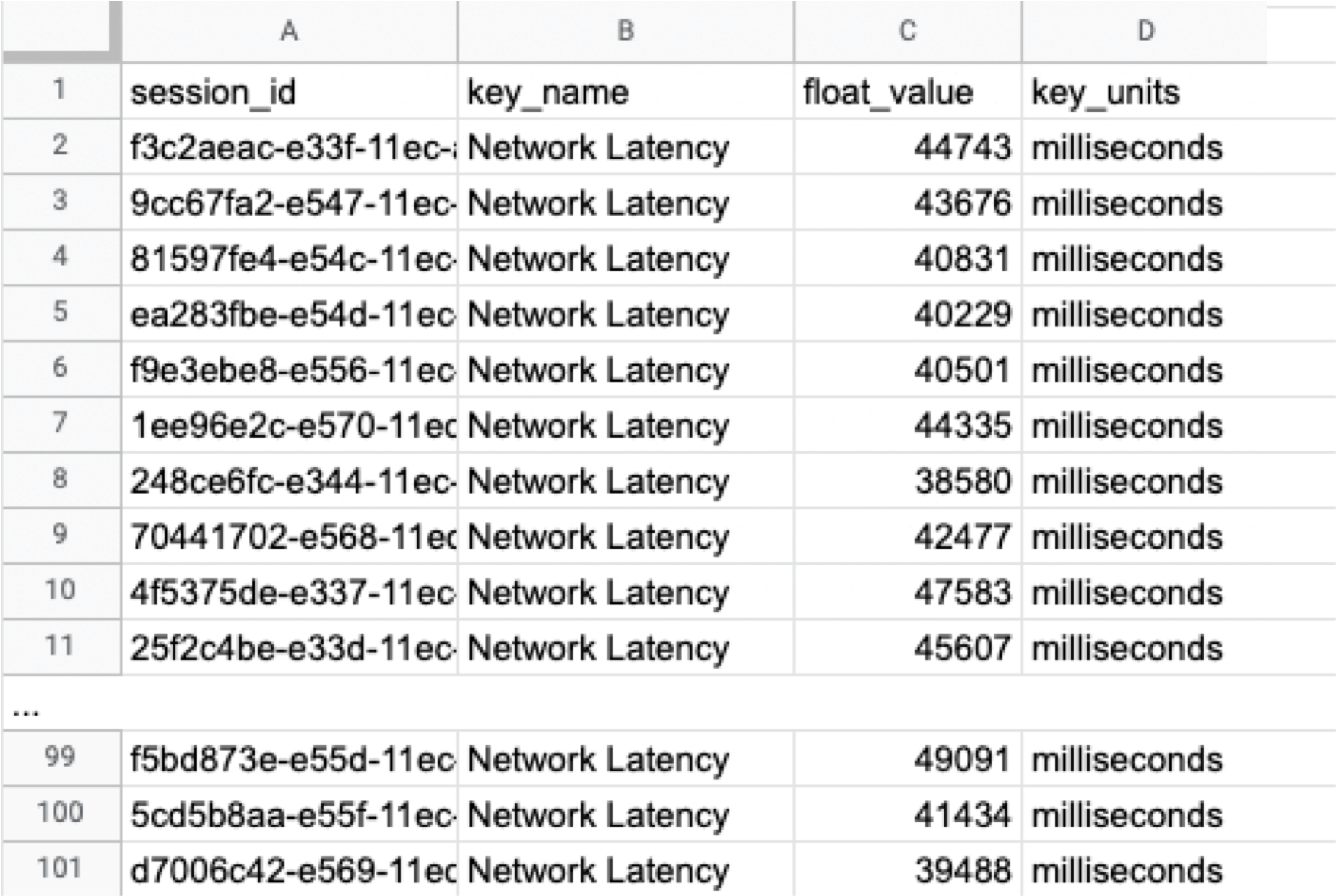
Read:

What we want to do next with these interval percentages is to find an optimal threshold that we can use to determine if a fixation has occur. Only so we will be capable to tell from the numbers what is normal and abnormal.Find an optimum threshold.
Alos read:
Accelerated Development with Data Science Insights for Enterprises..
Continuous monitoring and random sample
population average / (upper critical point - population average) = 43.8s / (52.6s - 43.8s) ≒ 5 %.Table: sample average and population norm
Read more:
Comparison and Prediction
1. Percentile
Also chit:
Creating regression account specifying percentiles (WEB UI)
Creating regression reports specifying percentiles (API)
curl -- location -- postulation POST 'https: // {{auth_token}} api-dev.headspin.io/v0/regression ' \ -- data-raw ' {`` a '': `` build:1.0 '', `` b '': `` build:2.0 '', “ centile ”: 50, “ limit '' :100, `` user_flow_name '': `` regression analysis ''} 'API Result:
2. Percentile Rank
Test and monitor website & amp; apps with our vast real local devices across the world..

3. Correlation and Prediction


Leverage digital experience monitoring capabilities for proactive resoluteness of app issues..
Summary
Shinji Kanai

![]()
Piali Mazumdar

![]()
Regression Intelligence hard-nosed guide for advanced users (Part 2)
4 Parts
-1280X720-Final-2.jpg)
Regression Intelligence practical guide for advanced users (Part 3)
Regression Intelligence practical guide for advanced users (Part 4)
Discover how HeadSpin can authorise your business with superior testing capabilities
![]()
![]()
![]()
![]()
![]()
![]()
![]()
![]()


![]()
![]()

Discover how HeadSpin can empower your business with superior testing capabilities
![]()
![]()
![]()
![]()
![]()
![]()
Discover how HeadSpin can empower your business with superior essay capabilities
![]()
![]()
![]()
![]()
![]()
![]()
Connet Now


![]()
![]()
![]()
![]()
![]()
![]()
![]()
Automate This With SUSA
Test Your App Autonomously


.png)